Visualization

Piccolo.jl provides visualization tools for analyzing optimization results. This guide covers plotting controls, states, and populations.

Setup

Visualization requires a Makie backend. We'll create a solved problem to work with:

using Piccolo
using CairoMakie
using Random
Random.seed!(42)

# Create and solve a simple qubit gate problem
H_drift = 0.5 * PAULIS[:Z]
H_drives = [PAULIS[:X], PAULIS[:Y]]
sys = QuantumSystem(H_drift, H_drives, [1.0, 1.0])

T = 10.0
N = 50
times = collect(range(0, T, length = N))
initial_controls = 0.1 * randn(2, N)
pulse = ZeroOrderPulse(initial_controls, times)
qtraj = UnitaryTrajectory(sys, pulse, GATES[:X])

# Lock the time grid to a uniform spacing so the ZOH stair plot has
# consistent step widths. Without this, the optimizer can vary Δt_k.
opts = PiccoloOptions(timesteps_all_equal = true, display = :silent)

qcp = SmoothPulseProblem(
    qtraj,
    N;
    Q = 100.0,
    R = 1e-2,
    ddu_bound = 1.0,
    piccolo_options = opts,
)
solve!(qcp; max_iter = 50, print_level = 1)

┌ Warning: Trajectory has timestep variable :Δt but no bounds on it.
│ Adding default lower bound of 0 to prevent negative timesteps.
│ 
│ Recommended: Add explicit bounds when creating the trajectory:
│   NamedTrajectory(...; Δt_bounds=(min, max))
│ Example:
│   NamedTrajectory(qtraj, N; Δt_bounds=(1e-3, 0.5))
│ 
│ Or use timesteps_all_equal=true in problem options to fix timesteps.
└ @ DirectTrajOpt.Problems ~/.julia/packages/DirectTrajOpt/2ZMae/src/problems.jl:66

******************************************************************************
This program contains Ipopt, a library for large-scale nonlinear optimization.
 Ipopt is released as open source code under the Eclipse Public License (EPL).
         For more information visit https://github.com/coin-or/Ipopt
******************************************************************************

    initializing optimizer...
      building evaluator: 3 integrators, 0 nonlinear constraints
      dynamics constraints: 588, nonlinear constraints: 0
        integrator 1 jacobian structure: 0.106s
        integrator 2 jacobian structure: 0.008s
        integrator 3 jacobian structure: 0.0s
      jacobian structure: 18816 nonzeros (0.126s)
        integrator 1 hessian structure: 0.01s
        integrator 2 hessian structure: 0.01s
        integrator 3 hessian structure: 0.002s
        computing objective hessian structure (CompositeObjective)...
          sub-objective 1 (KnotPointObjective): 0.16s
          sub-objective 2 (QuadraticRegularizer): 0.144s
          sub-objective 3 (QuadraticRegularizer): 0.0s
          sub-objective 4 (QuadraticRegularizer): 0.0s
          sub-objective 5 (NullObjective): 0.003s
        objective hessian structure: 0.33s
      hessian structure: 19344 nonzeros (0.353s)
      linear index maps built (0.005s)
      evaluator ready (total: 0.542s)
    evaluator created (0.742s)
    NL constraint bounds extracted (0.01s)
    NLP block data built (0.0s)
    Ipopt optimizer configured (0.005s)
    variables set (0.092s)
        applying constraint: timesteps all equal constraint
        applying constraint: initial value of Ũ⃗
        applying constraint: initial value of u
        applying constraint: final value of u
        applying constraint: bounds on Ũ⃗
        applying constraint: bounds on u
        applying constraint: bounds on du
        applying constraint: bounds on ddu
        applying constraint: bounds on Δt
        applying constraint: time consistency constraint (t_{k+1} = t_k + Δt_k)
        applying constraint: initial time t₁ = 0
    linear constraints added: 11 (0.293s)
    optimizer initialization complete (total: 1.154s)
[ Info: Loaded cached trajectory from visualization_unitary_f5c089b.jld2

Inspect the resulting fidelity:

fidelity(qcp)

0.9999965881970798

Pulse Plotting

plot_pulse renders any AbstractPulse with type-appropriate visuals (step functions for ZeroOrderPulse, line segments for LinearSplinePulse, smooth curves with knots for CubicSplinePulse, dense samples for analytic / FunctionPulse types). For per-pulse-type construction and rendering examples — including hardware bounds, tangent whiskers, theming, and the :stacked vs :overlay layouts — see the Pulses concept page. This guide focuses on plotting workflow pieces specific to optimization output.

Plot directly from a QuantumControlProblem

After solving, plot_pulse(qcp) extracts the optimized pulse and renders it in one call. Per-drive labels default to "<drive_name>_<i>". Pass bounds=true to shade hardware bounds derived from the system, and components=[:du, :ddu] to stack the derivative trajectories beneath the pulse with their own bounded panels (set component_bounds=true to read bounds from the NamedTrajectory).

fig = plot_pulse(qcp; title = "Optimized Pulse")

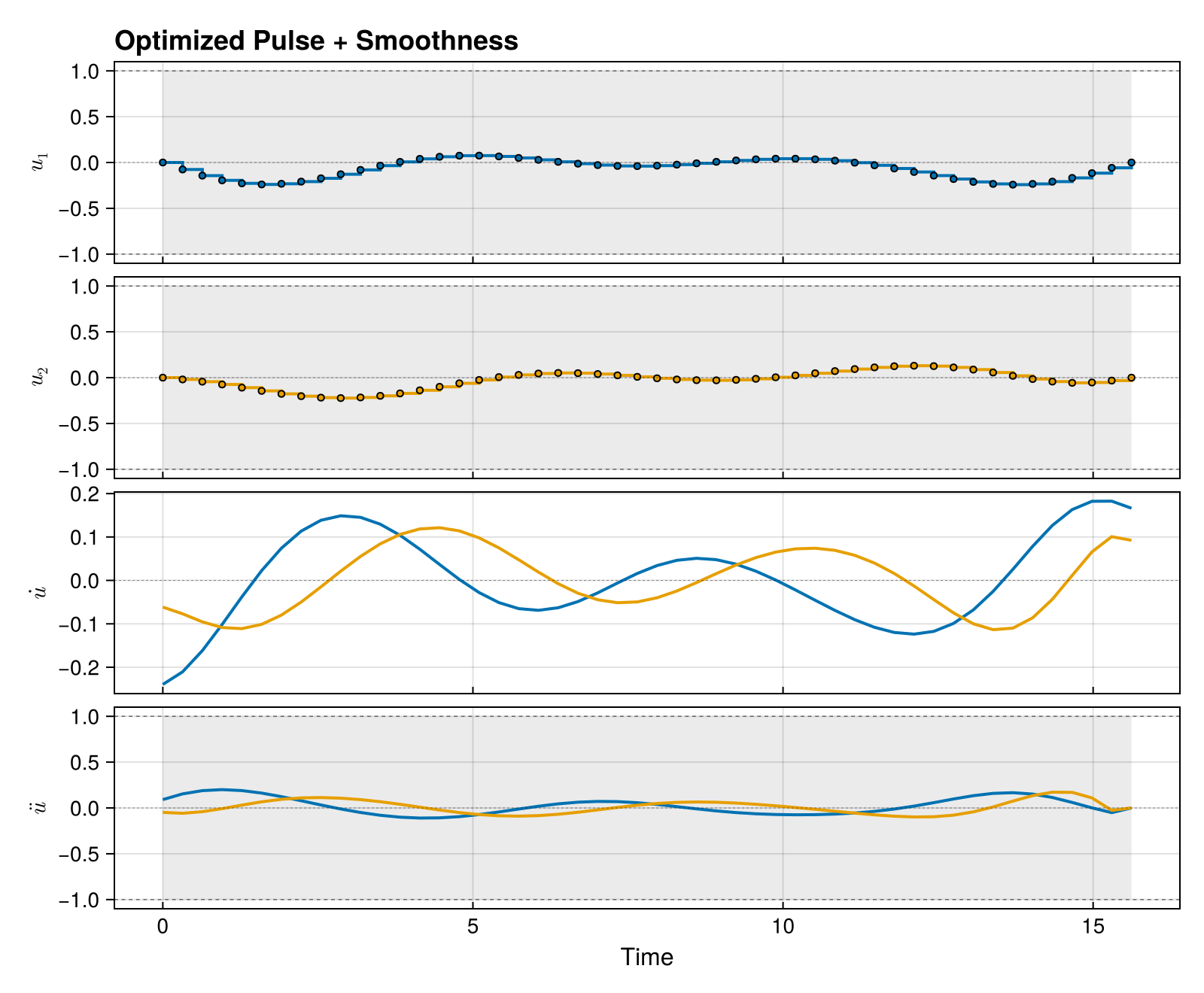
Add hardware bounds and the smoothness derivatives:

fig = plot_pulse(
    qcp;
    title = "Optimized Pulse + Smoothness",
    bounds = true,
    components = [:du, :ddu],
    component_bounds = true,
)

Manual extract + plot

If you need to manipulate the pulse before plotting (e.g. resample, convert to a different pulse type), reconstruct it explicitly. The higher-level plot_pulse(qcp; ...) calls do this internally.

optimized_traj = get_trajectory(qcp)
optimized_pulse = ZeroOrderPulse(optimized_traj)
fig = plot_pulse(optimized_pulse; title = "Optimized Pulse")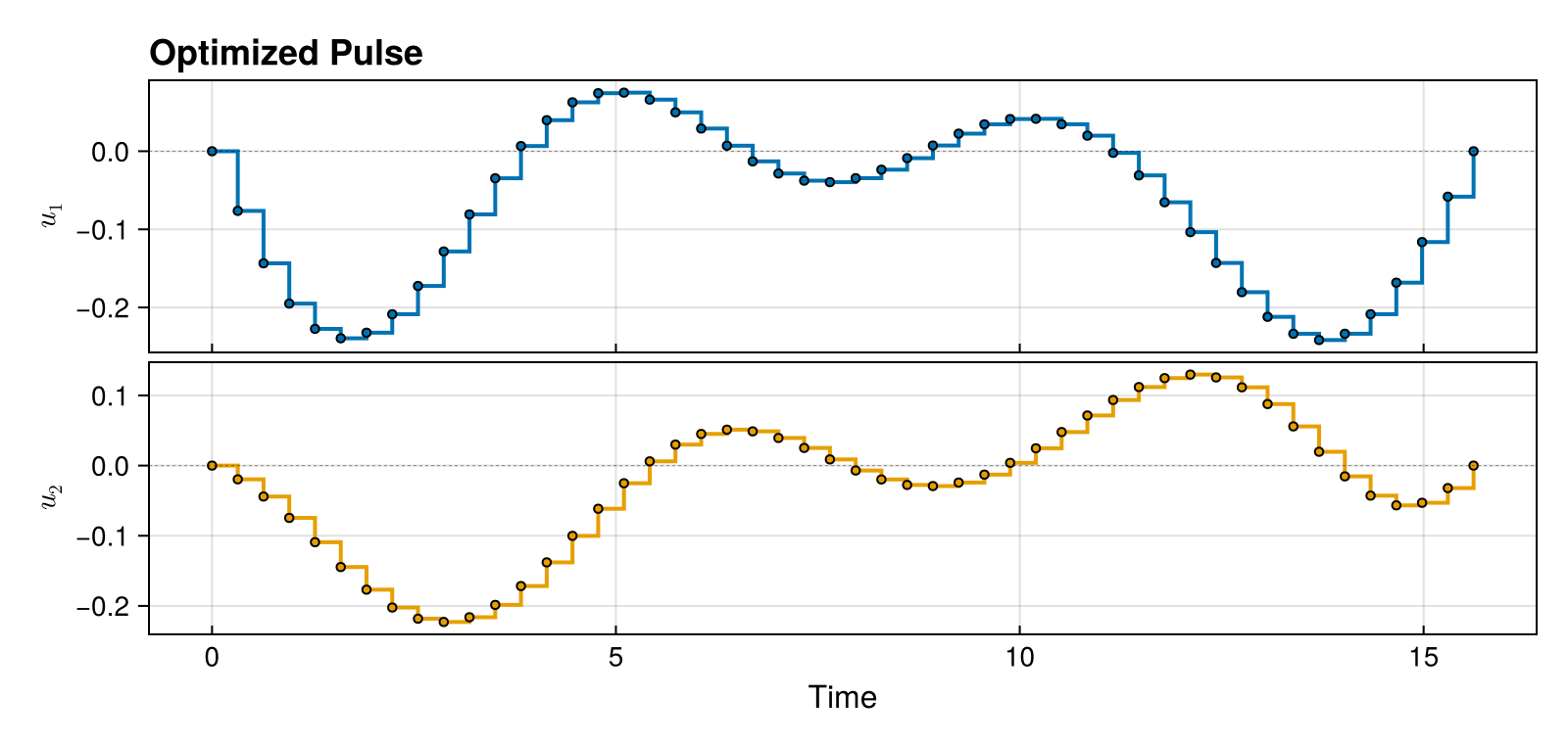

Basic Trajectory Plotting

The plot function from NamedTrajectories.jl plots trajectory components directly. This is useful for inspecting the raw optimization state, but it is not a faithful picture of the pulse you'll actually play on hardware.

Plot Controls

traj = get_trajectory(qcp)
fig = plot(traj, [:u])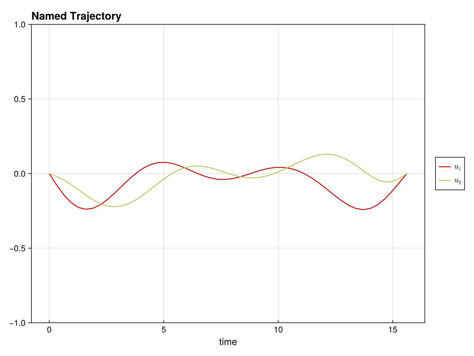

Plot Controls and Derivatives

fig = plot(traj, [:u, :du, :ddu])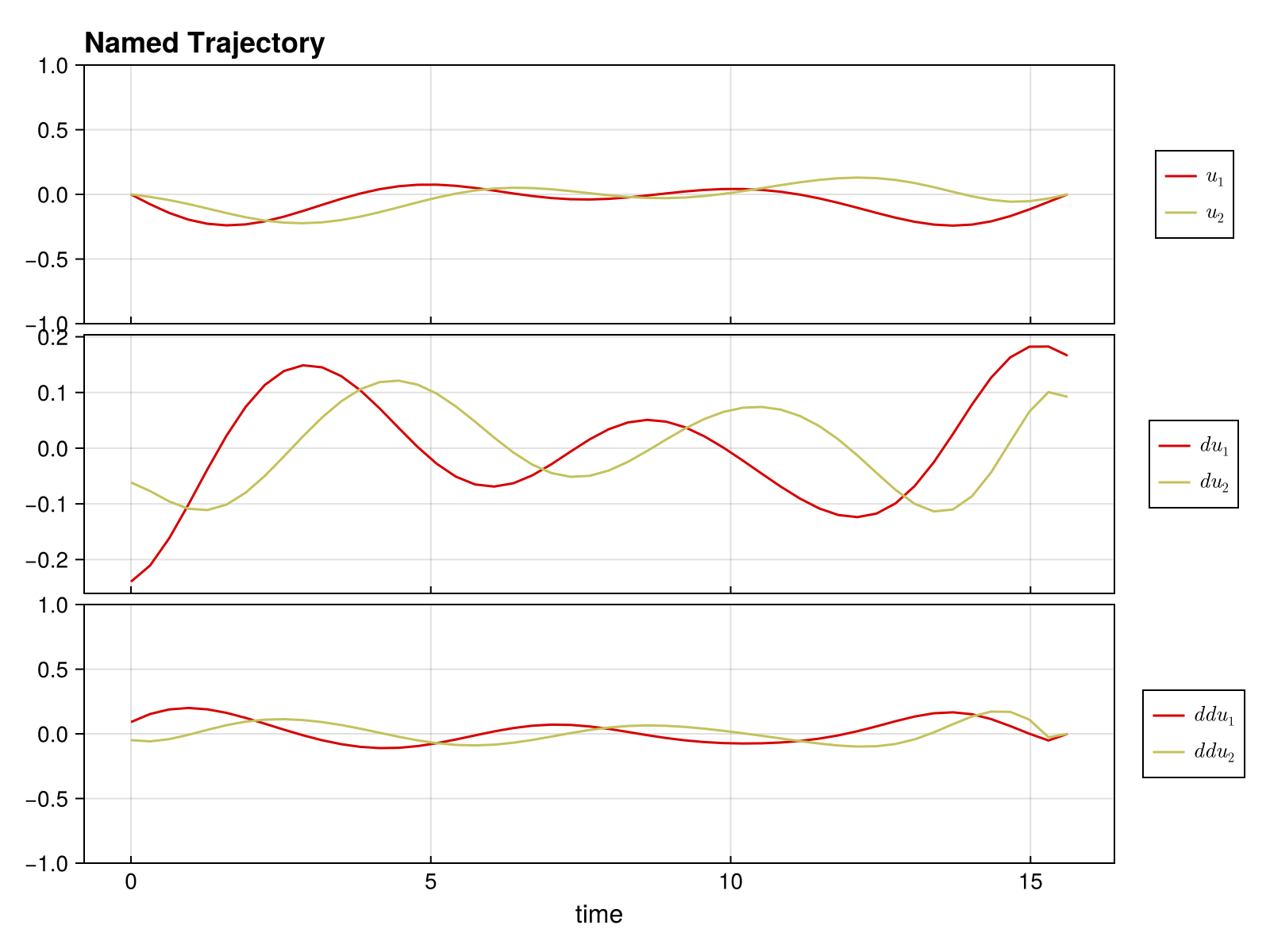

Quantum-Specific Plots

Unitary Populations

For UnitaryTrajectory, visualize how state populations evolve during the gate:

fig = plot_unitary_populations(traj)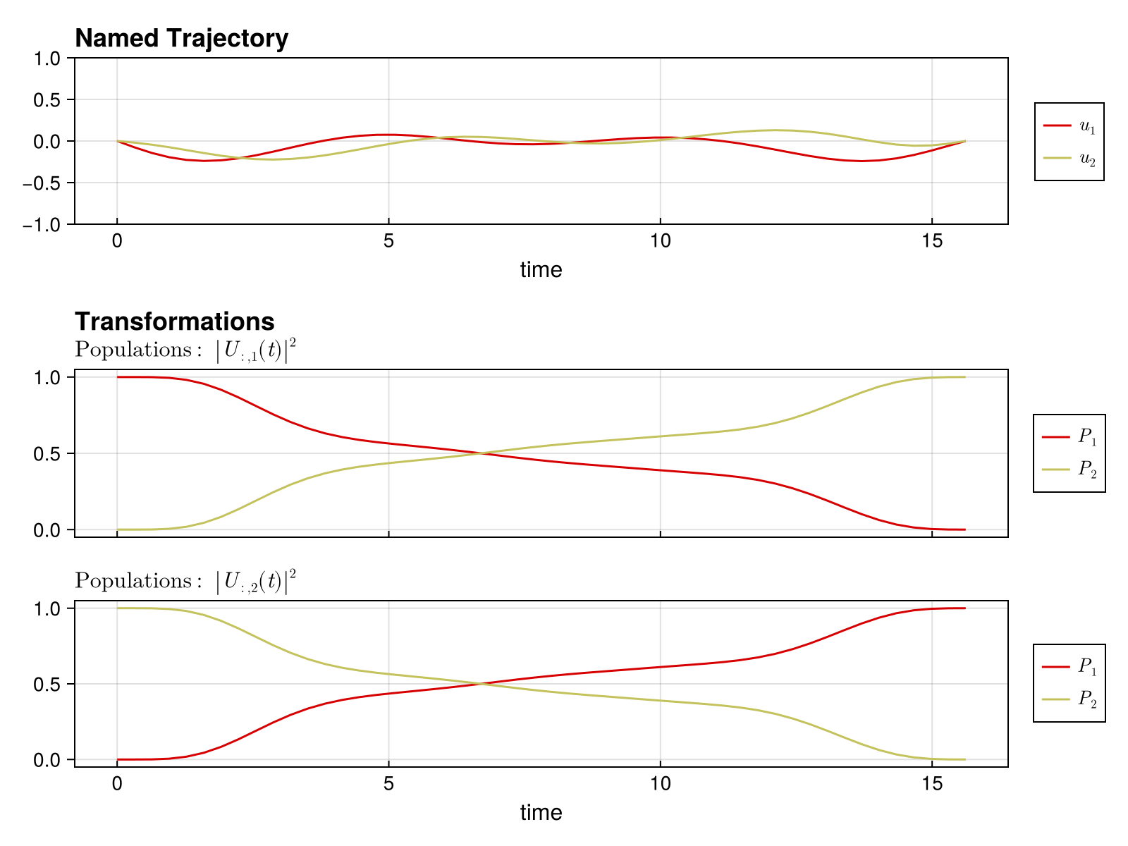

Ket State Populations

For KetTrajectory, use plot_state_populations. Set up and solve a |0⟩ → |1⟩ transfer on the same sys. As in the unitary example above, pin the time grid with timesteps_all_equal = true so the population plot has a uniform time axis:

ψ_init = ComplexF64[1.0, 0.0]
ψ_goal = ComplexF64[0.0, 1.0]

pulse_ket = ZeroOrderPulse(0.1 * randn(2, N), times)
qtraj_ket = KetTrajectory(sys, pulse_ket, ψ_init, ψ_goal)
qcp_ket = SmoothPulseProblem(
    qtraj_ket,
    N;
    Q = 100.0,
    R = 1e-2,
    ddu_bound = 1.0,
    piccolo_options = PiccoloOptions(timesteps_all_equal = true, verbose = false),
)
solve!(qcp_ket; max_iter = 50, print_level = 1)

┌ Warning: Trajectory has timestep variable :Δt but no bounds on it.
│ Adding default lower bound of 0 to prevent negative timesteps.
│ 
│ Recommended: Add explicit bounds when creating the trajectory:
│   NamedTrajectory(...; Δt_bounds=(min, max))
│ Example:
│   NamedTrajectory(qtraj, N; Δt_bounds=(1e-3, 0.5))
│ 
│ Or use timesteps_all_equal=true in problem options to fix timesteps.
└ @ DirectTrajOpt.Problems ~/.julia/packages/DirectTrajOpt/2ZMae/src/problems.jl:66

******************************************************************************
This program contains Ipopt, a library for large-scale nonlinear optimization.
 Ipopt is released as open source code under the Eclipse Public License (EPL).
         For more information visit https://github.com/coin-or/Ipopt
******************************************************************************

    initializing optimizer...
      building evaluator: 3 integrators, 0 nonlinear constraints
      dynamics constraints: 392, nonlinear constraints: 0
        integrator 1 jacobian structure: 0.132s
        integrator 2 jacobian structure: 0.011s
        integrator 3 jacobian structure: 0.0s
      jacobian structure: 9408 nonzeros (0.16s)
        integrator 1 hessian structure: 0.013s
        integrator 2 hessian structure: 0.013s
        integrator 3 hessian structure: 0.575s
        computing objective hessian structure (CompositeObjective)...
          sub-objective 1 (KnotPointObjective): 0.2s
          sub-objective 2 (QuadraticRegularizer): 0.179s
          sub-objective 3 (QuadraticRegularizer): 0.0s
          sub-objective 4 (QuadraticRegularizer): 0.0s
          sub-objective 5 (NullObjective): 0.004s
        objective hessian structure: 0.416s
      hessian structure: 10956 nonzeros (1.017s)
      linear index maps built (0.004s)
      evaluator ready (total: 1.266s)
    evaluator created (1.518s)
    NL constraint bounds extracted (0.015s)
    NLP block data built (0.0s)
    Ipopt optimizer configured (0.005s)
    variables set (0.072s)
        applying constraint: timesteps all equal constraint
        applying constraint: initial value of ψ̃
        applying constraint: initial value of u
        applying constraint: final value of u
        applying constraint: bounds on ψ̃
        applying constraint: bounds on u
        applying constraint: bounds on du
        applying constraint: bounds on ddu
        applying constraint: bounds on Δt
        applying constraint: time consistency constraint (t_{k+1} = t_k + Δt_k)
        applying constraint: initial time t₁ = 0
    linear constraints added: 11 (0.304s)
    optimizer initialization complete (total: 1.914s)
[ Info: Loaded cached trajectory from visualization_ket_46df54b.jld2

Plot the populations:

traj_ket = get_trajectory(qcp_ket)
fig = plot_state_populations(traj_ket)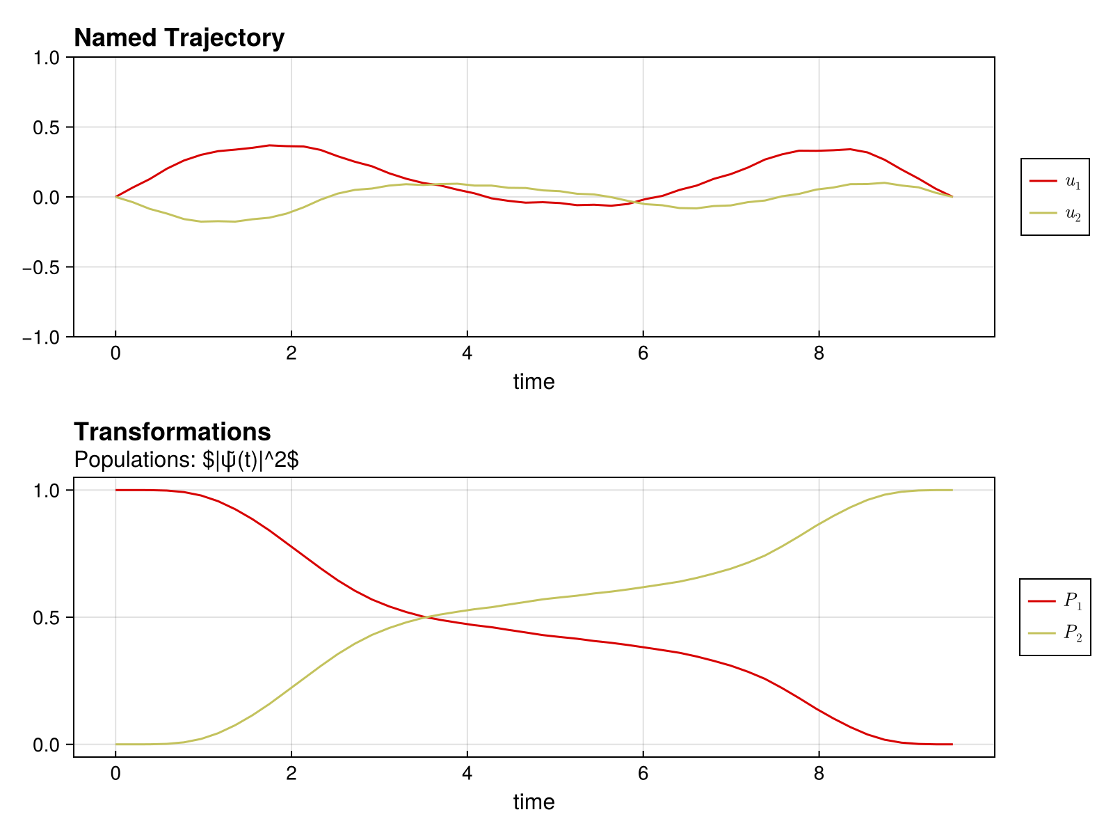

Bloch Sphere Visualization

When QuantumToolbox.jl is loaded, plot_bloch renders a two-level state trajectory on the Bloch sphere. The path connects the Bloch vector at every timestep; pass index=k to also drop a vector arrow at frame k.

using QuantumToolbox
fig = plot_bloch(traj_ket)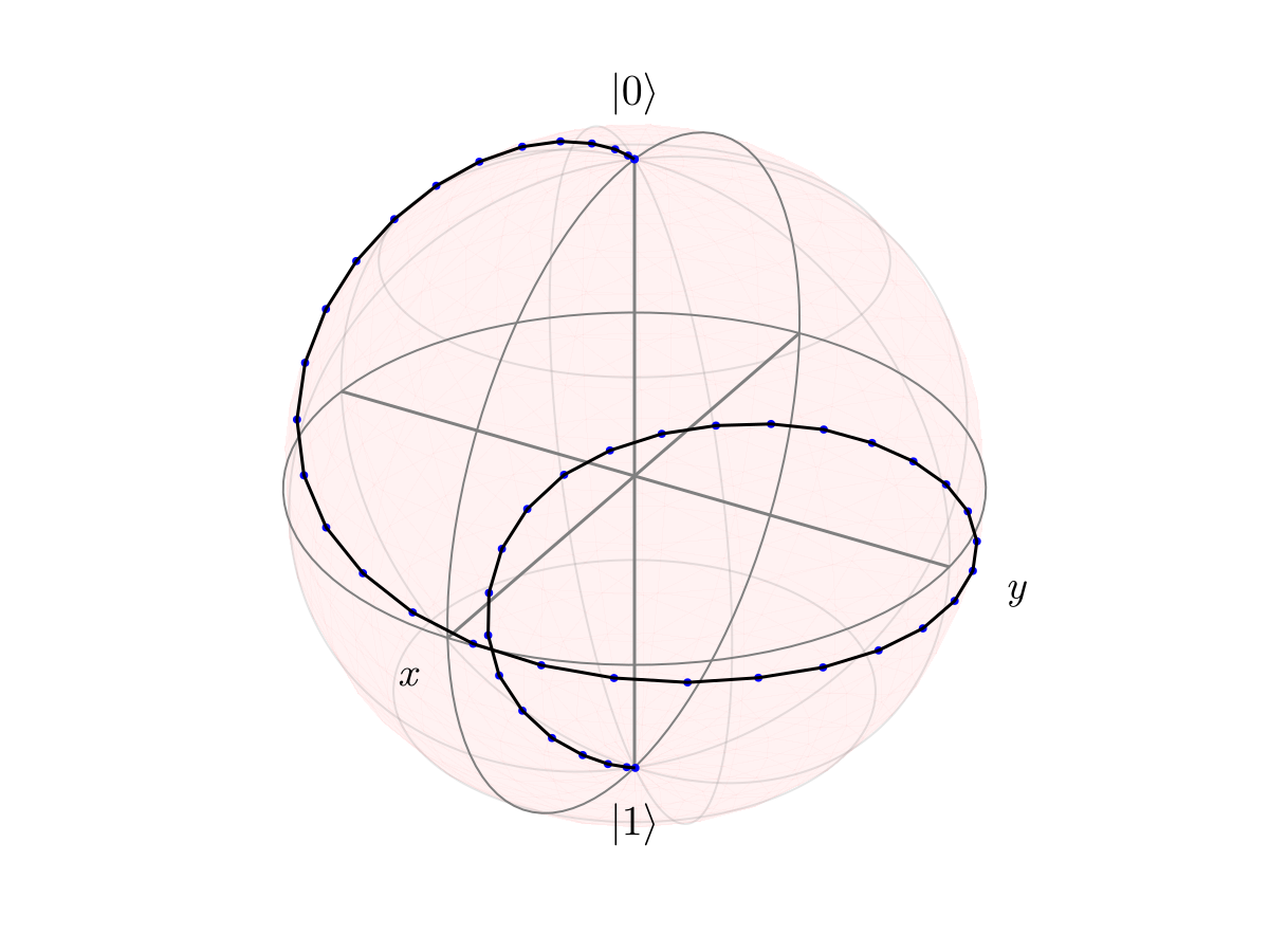

Show a vector arrow at a specific timestep:

fig = plot_bloch(traj_ket; index = N)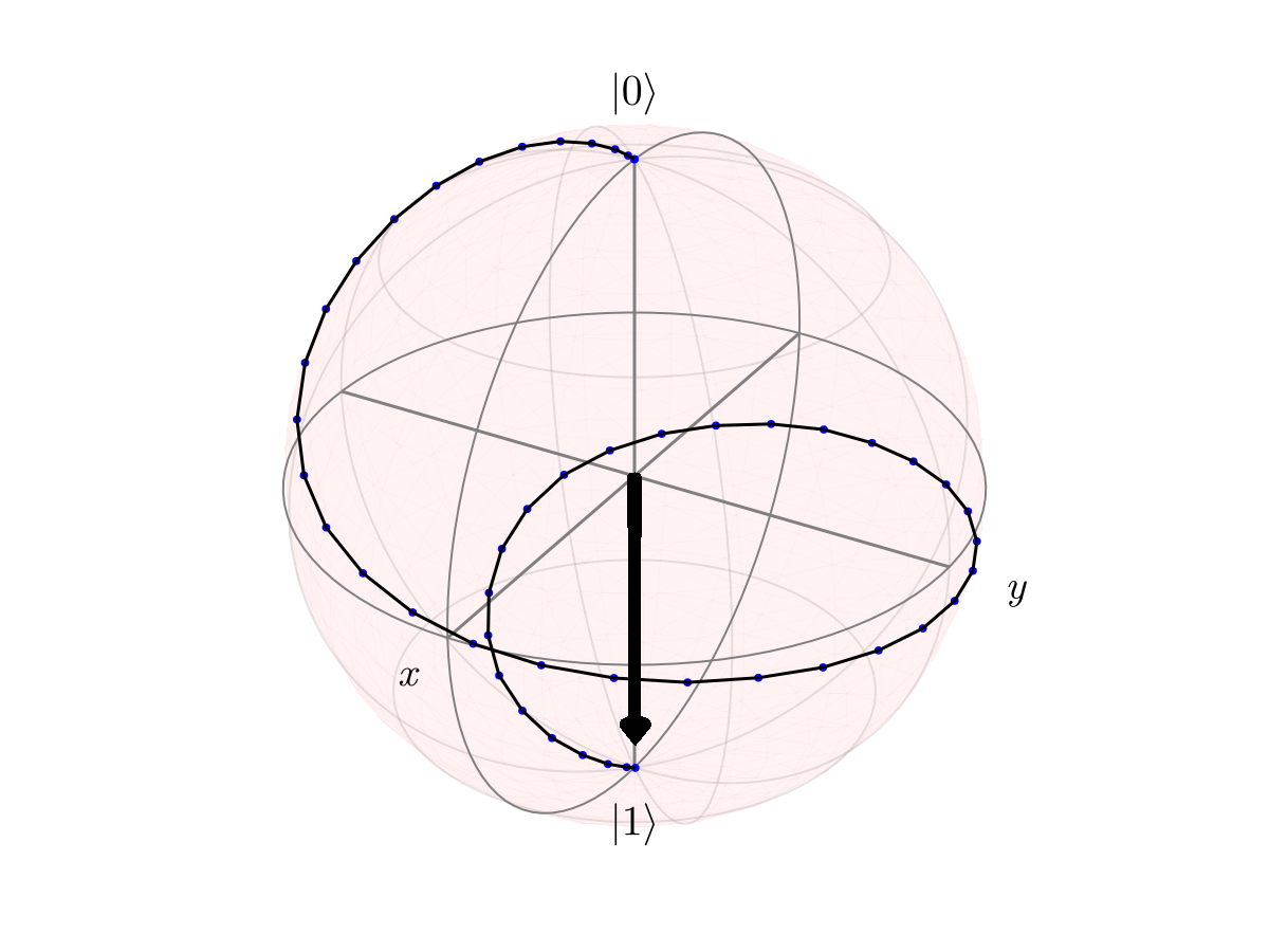

For multi-level systems, restrict to the qubit subspace via subspace=1:2. For density-matrix trajectories, pass state_name=:ρ̃⃗, state_type=:density.

Wigner Function Visualization

For bosonic / oscillator systems, plot_wigner(traj, idx) renders the Wigner quasi-probability distribution at a chosen timestep. To keep this guide fast we build a small synthetic trajectory of coherent states rotating in phase space — no solver involved — to illustrate the call:

dim_cavity = 20
N_cav = 30
ω_cav = 2π
times_cav = range(0, 2π / ω_cav, length = N_cav)
cavity_kets = [coherent(dim_cavity, 1.5 * exp(im * ω_cav * t)).data for t in times_cav]
traj_cavity = NamedTrajectory((
    ψ̃ = hcat(ket_to_iso.(cavity_kets)...),
    Δt = fill(step(times_cav), N_cav),
),)

fig = plot_wigner(traj_cavity, 1; xvec = -3:0.1:3, yvec = -3:0.1:3)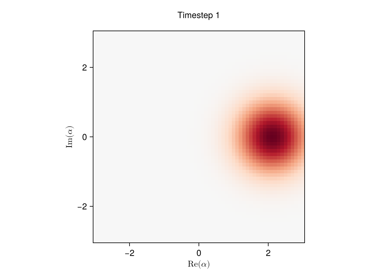

A single static frame can't show the orbital motion (the coherent state at t = 0 and t = 2π/ω_cav sits at the same phase-space point). Use animate_wigner with mode = :record to write a .gif next to the generated page and embed it. Interactive :inline playback requires GLMakie, which the docs build doesn't load.

animate_wigner(
    traj_cavity;
    mode = :record,
    filename = "wigner_cavity.gif",
    fps = 12,
    xvec = -3:0.1:3,
    yvec = -3:0.1:3,
)

Bloch evolution can be animated the same way with animate_bloch(traj_ket; mode = :record, filename = "bloch.gif").

IQ pairs (plot_pulse_IQ)

For 4-drive pulses interpreted as two IQ pairs — drive (ΩI, ΩQ) and displacement (αI, αQ) — plot_pulse_IQ renders each pair on its own row along with the magnitude envelope. Typical view for cat-qubit / oscillator control where both the drive and displacement are complex-valued.

T_iq = 50.0
Ω_max = 0.5
α_max = 0.3
σ = T_iq / 6
pulse_iq = GaussianPulse([Ω_max, 0.7 * Ω_max, α_max, 0.7 * α_max], σ, T_iq)

fig = plot_pulse_IQ(pulse_iq; title = "IQ view (Ω, α)")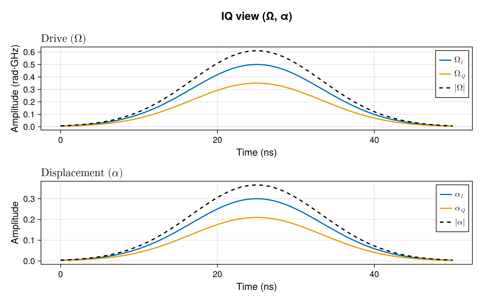

Magnitude + phase (plot_pulse_phases)

Same 4-drive structure, polar form: magnitude and unwrapped phase for the drive on the top row, displacement on the bottom row. Phase is masked to NaN wherever the corresponding amplitude is below 1% of its peak (configurable via phase_threshold) since atan(Q, I) is numerically meaningless in the near-zero region.

fig = plot_pulse_phases(pulse_iq; title = "Polar view (|·|, ∠·)")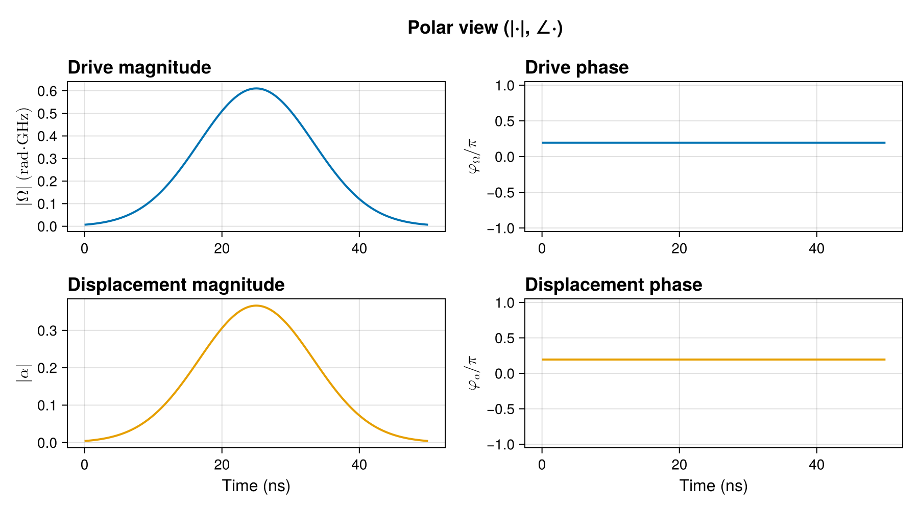

Custom Plotting

For full control, extract trajectory data and use Makie directly.

Manual Control Plots

plot_times = cumsum([0; get_timesteps(traj)])[1:(end-1)]

fig = Figure(size = (800, 400))
ax = Axis(fig[1, 1], xlabel = "Time", ylabel = "Control Amplitude")

for i = 1:size(traj[:u], 1)
    lines!(ax, plot_times, traj[:u][i, :], label = "Drive $i", linewidth = 2)
end

axislegend(ax, position = :rt)
fig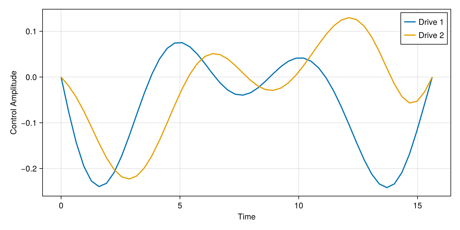

Subplot Layouts

fig = Figure(size = (1000, 500))

# Controls
ax1 = Axis(fig[1, 1], xlabel = "Time", ylabel = "Amplitude", title = "Controls")
lines!(ax1, plot_times, traj[:u][1, :], label = "u_x", linewidth = 2)
lines!(ax1, plot_times, traj[:u][2, :], label = "u_y", linewidth = 2)
axislegend(ax1, position = :rt)

# Derivatives
ax2 = Axis(fig[1, 2], xlabel = "Time", ylabel = "Derivative", title = "Control Derivatives")
lines!(ax2, plot_times, traj[:du][1, :], label = "du_x", linewidth = 2)
lines!(ax2, plot_times, traj[:du][2, :], label = "du_y", linewidth = 2)
axislegend(ax2, position = :rt)

fig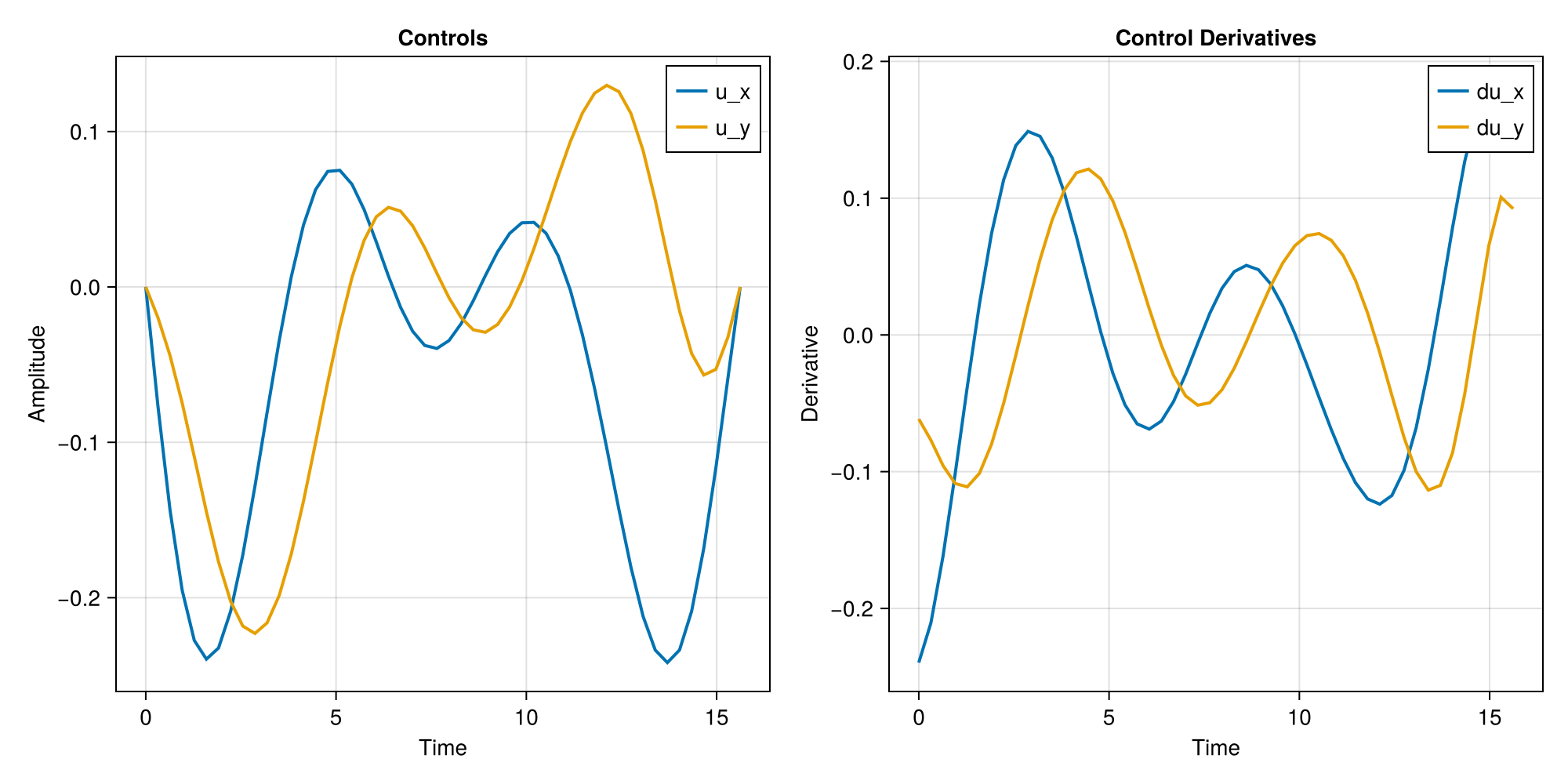

Phase Space Plot

fig = Figure(size = (500, 500))
ax = Axis(fig[1, 1], xlabel = "u_x", ylabel = "u_y", title = "Control Phase Space")
lines!(ax, traj[:u][1, :], traj[:u][2, :], linewidth = 2)
scatter!(
    ax,
    [traj[:u][1, 1]],
    [traj[:u][2, 1]],
    color = :green,
    markersize = 15,
    label = "Start",
)
scatter!(
    ax,
    [traj[:u][1, end]],
    [traj[:u][2, end]],
    color = :red,
    markersize = 15,
    label = "End",
)
axislegend(ax, position = :rt)
fig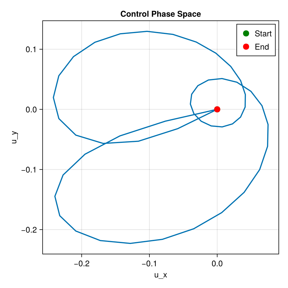

Fidelity Evolution

Track fidelity during the pulse:

using LinearAlgebra

U_goal = GATES[:X]
fidelities = Float64[]
for k = 1:size(traj[:Ũ⃗], 2)
    U_k = iso_vec_to_operator(traj[:Ũ⃗][:, k])
    F_k = abs(tr(U_goal' * U_k))^2 / sys.levels^2
    push!(fidelities, F_k)
end

fig = Figure(size = (800, 300))
ax = Axis(fig[1, 1], xlabel = "Timestep", ylabel = "Fidelity")
lines!(ax, 1:length(fidelities), fidelities, linewidth = 2)
hlines!(ax, [0.99], color = :red, linestyle = :dash, label = "99% target")
axislegend(ax, position = :rb)
fig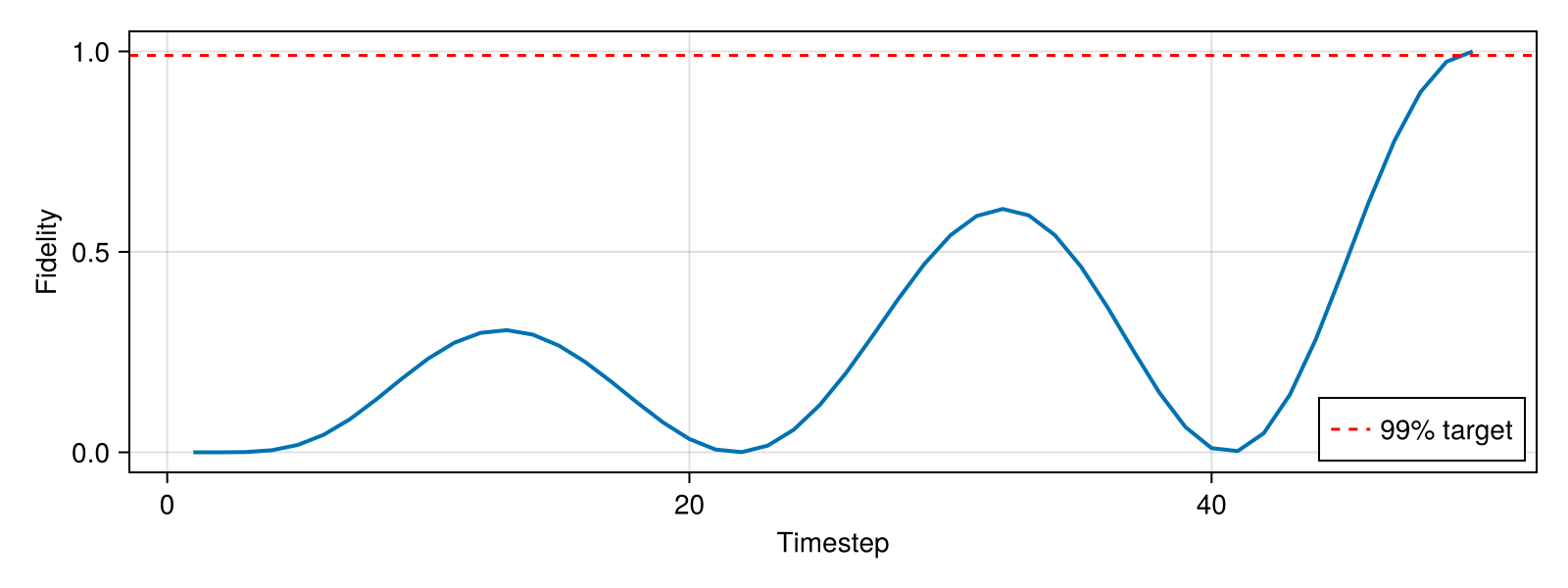

Comparing Solutions

Compare solutions with different regularization weights:

fig = Figure(size = (800, 400))
ax = Axis(fig[1, 1], xlabel = "Time", ylabel = "u_x", title = "Effect of Regularization")

for (R, label) in [(1e-3, "R=1e-3"), (1e-2, "R=1e-2"), (1e-1, "R=1e-1")]
    pulse_r = ZeroOrderPulse(0.1 * randn(2, N), times)
    qtraj_r = UnitaryTrajectory(sys, pulse_r, GATES[:X])
    qcp_r = SmoothPulseProblem(qtraj_r, N; Q = 100.0, R = R, ddu_bound = 1.0)
    solve!(
        qcp_r;
        max_iter = 50,
        verbose = false,
        print_level = 1,
    )
    traj_r = get_trajectory(qcp_r)
    t_r = cumsum([0; get_timesteps(traj_r)])[1:(end-1)]
    lines!(ax, t_r, traj_r[:u][1, :], label = label, linewidth = 2)
end

axislegend(ax, position = :rt)
fig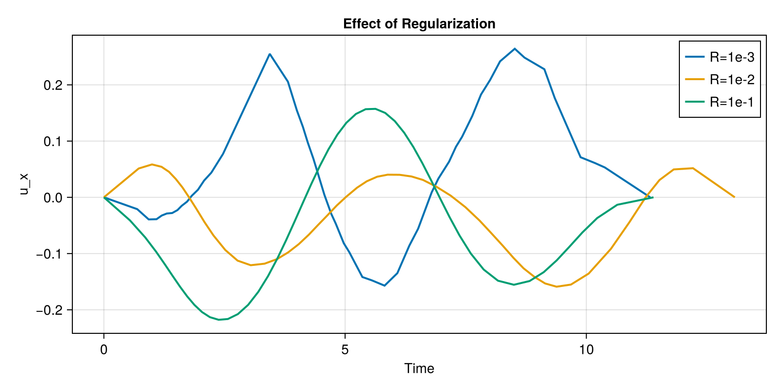

Saving Figures

# PNG (raster)
# save("controls.png", fig)

# PDF (vector graphics)
# save("controls.pdf", fig)

# SVG (vector graphics)
# save("controls.svg", fig)

Plotting Tips

1. Use Appropriate Resolution

For publications, use high-res settings:

fig_hires = Figure(size = (1200, 800), fontsize = 14)

2. Use Consistent Colors

colors = Makie.wong_colors()

3. Show Drive Bounds

bound = 1.0
fig = Figure(size = (800, 300))
ax = Axis(fig[1, 1], xlabel = "Time", ylabel = "Amplitude")
band!(
    ax,
    plot_times,
    -bound * ones(length(plot_times)),
    bound * ones(length(plot_times)),
    color = (:gray, 0.2),
    label = "Bounds",
)
lines!(ax, plot_times, traj[:u][1, :], label = "u_x", linewidth = 2)
axislegend(ax, position = :rt)
fig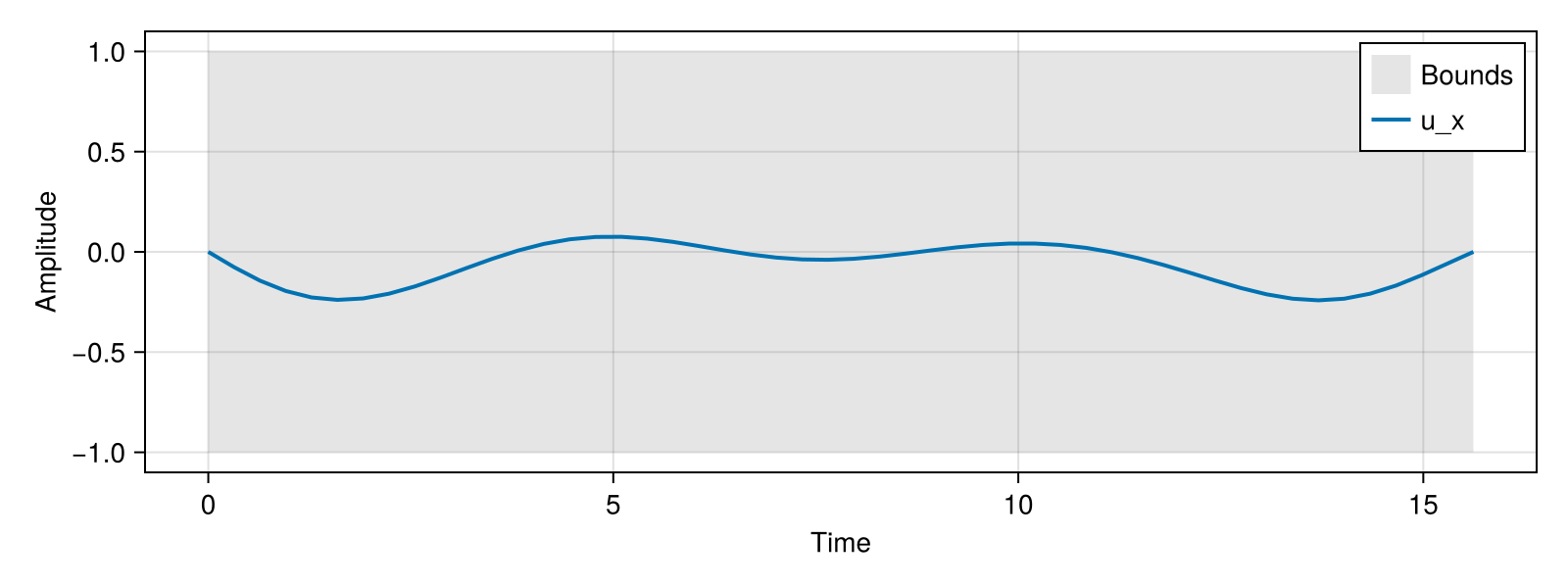

See Also

• Visualizations API - Complete API reference
• Problem Templates - Generating solutions to plot
• Trajectories - Understanding trajectory structure

This page was generated using Literate.jl.