Quickstart Guide

Welcome to DirectTrajOpt.jl! This guide will get you up and running in minutes.

What is DirectTrajOpt?

DirectTrajOpt.jl solves trajectory optimization problems - finding optimal control sequences that drive a dynamical system from an initial state to a goal state while minimizing a cost function.

Installation

First, install the package:

using Pkg
Pkg.add("DirectTrajOpt")

You'll also need NamedTrajectories.jl for defining trajectories:

using DirectTrajOpt
using NamedTrajectories
using LinearAlgebra
using CairoMakie

A Minimal Example

Let's solve a simple problem: drive a 2D system from [0, 0] to [1, 0] with minimal control effort.

Step 1: Define the Trajectory

A trajectory contains your states, controls, and time information:

N = 50  # number of time steps
traj = NamedTrajectory(
    (
        x = randn(2, N),    # 2D state
        u = randn(1, N),    # 1D control
        Δt = fill(0.1, N),   # time step
    );
    timestep = :Δt,
    controls = :u,
    initial = (x = [0.0, 0.0],),
    final = (x = [1.0, 0.0],),
    bounds = (Δt = (0.05, 0.2), u = 1.0),
)

N = 50, (x = 1:2, u = 3:3, → Δt = 4:4)

Step 2: Define the Dynamics

Specify how your system evolves. For bilinear dynamics ẋ = (G₀ + u₁G₁) x:

G_drift = [-0.1 1.0; -1.0 -0.1]   # drift term
G_drives = [[0.0 1.0; 1.0 0.0]]   # control term
G = u -> G_drift + sum(u .* G_drives)

integrator = BilinearIntegrator(G, :x, :u, traj)

BilinearIntegrator: :x = exp(Δt G(:u)) :x  (dim = 2)

Step 3: Define the Objective

What do we want to minimize? Let's penalize control effort:

obj = QuadraticRegularizer(:u, traj, 1.0)

QuadraticRegularizer on :u (R = [1.0], all)

Step 4: Create and Solve

Combine everything into a problem and solve:

prob = DirectTrajOptProblem(traj, obj, integrator)

DirectTrajOptProblem
  Trajectory
    Timesteps: 50
    Duration:  4.9
    Knot dim:  4
    Variables: x (2), u (1), Δt (1)
    Controls:  u, Δt
  Objective: QuadraticRegularizer on :u (R = [1.0], all)
  Dynamics (1 integrators)
    BilinearIntegrator: :x = exp(Δt G(:u)) :x  (dim = 2)
  Constraints (4 total: 2 equality, 2 bounds)
    EqualityConstraint: "initial value of x"
    EqualityConstraint: "final value of x"
    BoundsConstraint: "bounds on Δt"
    BoundsConstraint: "bounds on u"

The problem summary shows the trajectory, objective, dynamics, and constraints:

prob

DirectTrajOptProblem
  Trajectory
    Timesteps: 50
    Duration:  4.9
    Knot dim:  4
    Variables: x (2), u (1), Δt (1)
    Controls:  u, Δt
  Objective: QuadraticRegularizer on :u (R = [1.0], all)
  Dynamics (1 integrators)
    BilinearIntegrator: :x = exp(Δt G(:u)) :x  (dim = 2)
  Constraints (4 total: 2 equality, 2 bounds)
    EqualityConstraint: "initial value of x"
    EqualityConstraint: "final value of x"
    BoundsConstraint: "bounds on Δt"
    BoundsConstraint: "bounds on u"

solve!(prob; max_iter = 100, verbose = false)

This is Ipopt version 3.14.19, running with linear solver MUMPS 5.8.2.

Number of nonzeros in equality constraint Jacobian...:      776
Number of nonzeros in inequality constraint Jacobian.:        0
Number of nonzeros in Lagrangian Hessian.............:     1254

Total number of variables............................:      196
                     variables with only lower bounds:        0
                variables with lower and upper bounds:      100
                     variables with only upper bounds:        0
Total number of equality constraints.................:       98
Total number of inequality constraints...............:        0
        inequality constraints with only lower bounds:        0
   inequality constraints with lower and upper bounds:        0
        inequality constraints with only upper bounds:        0

iter    objective    inf_pr   inf_du lg(mu)  ||d||  lg(rg) alpha_du alpha_pr  ls
   0  1.2088135e-01 3.72e+00 2.10e-08   0.0 0.00e+00    -  0.00e+00 0.00e+00   0
   1  1.5925520e-01 1.71e-01 1.36e+00  -1.3 2.93e+00    -  9.68e-01 1.00e+00h  1

Number of Iterations....: 2

Number of objective function evaluations             = 3
Number of objective gradient evaluations             = 3
Number of equality constraint evaluations            = 3
Number of inequality constraint evaluations          = 0
Number of equality constraint Jacobian evaluations   = 2
Number of inequality constraint Jacobian evaluations = 0
Number of Lagrangian Hessian evaluations             = 2
Total seconds in IPOPT                               = 6.734

EXIT: Invalid number in NLP function or derivative detected.

Step 5: Access the Solution

Let's look at the results.

plot(prob.trajectory)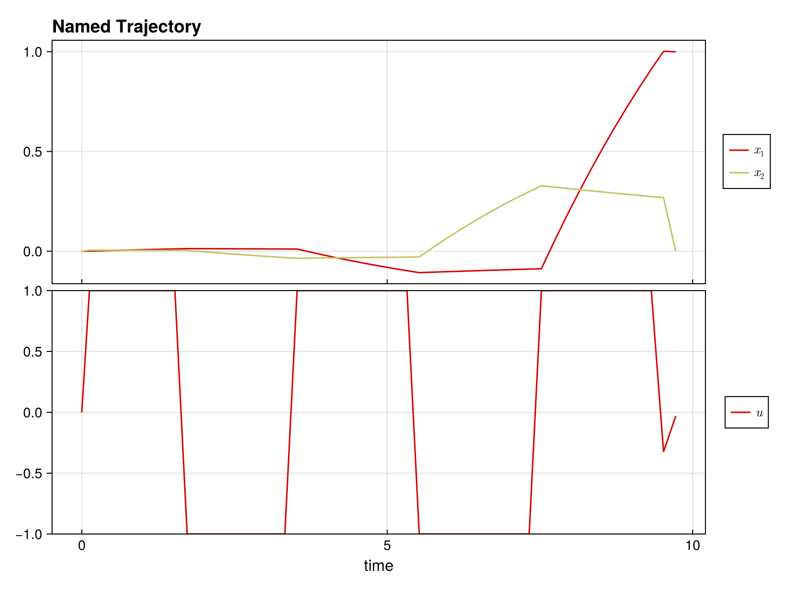

The optimized trajectory is stored in prob.trajectory:

println("Final state: ", prob.trajectory.x[:, end])
println("Control norm: ", norm(prob.trajectory.u))

Final state: [1.0, 0.0]
Control norm: 4.463206717820474

What You Can Do

Multiple objectives: Combine regularization, minimum time, terminal costs
Flexible dynamics: Linear, bilinear, time-dependent systems
Add constraints: Bounds, path constraints, custom nonlinear constraints
Smooth controls: Penalize derivatives for smooth, implementable controls
Free time: Optimize trajectory duration

This page was generated using Literate.jl.